Optimization#
Given that the main purpose of the SigmaEpsilon ecosystem is to facilitate structural optimization, this submodule needs no further elaboration, as having a capable optimization toolkit is essential for the project. The overarching approach is to utilize third-party solutions whenever feasible, though we also provide essential solutions when necessary or fill in the gaps wherever required.
.. note:: Most of the classes for optimization rely on other classes like :class:`~sigmaepsilon.math.function.function.Function` or :class:`~sigmaepsilon.math.function.relation.Relation`. Before you proceed forward, it might be a good idea to check them out first :ref:`hereLinear Programming (LP)#
📖 Linear Programming API Reference.
The library offers a solver for a wide range of linear optimization problems, including continuous, integer and mixed-integer problems. The LinearProgrammingProblem class uses the linprog module from SciPy (which eventually calls the HIGHS solver) for the solution, combined with the power of SymPy for being able to pose problems directly in symbolic form. The class handles all the preprocessing required to bring the problem into the form required by SciPy.
First, import some stuff. Note that the notebook requires matplotlib to be installed.
[1]:
from sigmaepsilon.math.function import Function, Relation
from sigmaepsilon.math.optimize import LinearProgrammingProblem as LPP
import sympy as sy
One of the great features of the optimization module is that it handles symbolic functions pretty well. Problems can be defined using SymPy expressions, or simple strings. To solve a problem, call the solve method, which returns an instance of scipy.optimize.OptimizeResult.
[2]:
x1, x2, x3, x4 = variables = sy.symbols(['x1', 'x2', 'x3', 'x4'])
obj = Function(3*x1 + 9*x3 + x2 + x4, variables=variables)
eq1 = Relation(x1 + 2*x3 + x4 - 4, variables=variables)
eq2 = Relation(x2 + x3 - x4 - 2, variables=variables)
bounds = [(0, None), (0, None), (0, None), (0, None)]
lpp = LPP(obj, [eq1, eq2], variables=variables, bounds=bounds)
solution = lpp.solve()
solution.x
[2]:
array([0., 6., 0., 4.])
[ ]:
solution
        message: Optimization terminated successfully. (HiGHS Status 7: Optimal)
        success: True
         status: 0
            fun: 10.0
              x: [ 0.000e+00  6.000e+00  0.000e+00  4.000e+00]
            nit: 0
          lower:  residual: [ 0.000e+00  6.000e+00  0.000e+00  4.000e+00]
                 marginals: [ 1.000e+00  0.000e+00  4.000e+00  0.000e+00]
          upper:  residual: [       inf        inf        inf        inf]
                 marginals: [ 0.000e+00  0.000e+00  0.000e+00  0.000e+00]
          eqlin:  residual: [ 0.000e+00  0.000e+00]
                 marginals: [ 2.000e+00  1.000e+00]
        ineqlin:  residual: []
                 marginals: []
 mip_node_count: 0
 mip_dual_bound: 0.0
        mip_gap: 0.0
[ ]:
type(solution)
scipy.optimize._optimize.OptimizeResult
If the bounds for the variables are all the same, you can afford to input a single bound:
[5]:
x1, x2, x3, x4 = variables = sy.symbols(['x1', 'x2', 'x3', 'x4'])
obj = Function(3*x1 + 9*x3 + x2 + x4, variables=variables)
eq1 = Relation(x1 + 2*x3 + x4 - 4, variables=variables)
eq2 = Relation(x2 + x3 - x4 - 2, variables=variables)
bounds = (0, None)
lpp = LPP(obj, [eq1, eq2], variables=variables, bounds=bounds)
lpp.solve().x
[5]:
array([0., 6., 0., 4.])
Furthermore, if all the bounds are in the form \(\geq\), you can omit the arguments for the parameter bounds, since it is the default value.
[6]:
variables = sy.symbols(['x1', 'x2', 'x3', 'x4'])
obj = Function("3*x1 + 9*x3 + x2 + x4", variables=variables)
eq1 = Relation("x1 + 2*x3 + x4 = 4", variables=variables)
eq2 = Relation("x2 + x3 - x4 = 2", variables=variables)
lpp = LPP(obj, [eq1, eq2], variables=variables)
lpp.solve().x
[6]:
array([0., 6., 0., 4.])
2d example with matplotlib#
Consider the following problem:
Setting up the problem is as follows.
[7]:
variables = sy.symbols(['x1', 'x2'])
f = Function("x1 + x2", variables=variables)
ieq1 = Relation("x1 >= 1", variables=variables)
ieq2 = Relation("x2 >= 1", variables=variables)
ieq3 = Relation("x1 + x2 <= 4", variables=variables)
bounds = [(0, None), (0, None)]  # x1 >= 0, x2 >= 0
lpp = LPP(f, [ieq1, ieq2, ieq3], variables=variables, bounds=bounds)
x = lpp.solve().x
print("The optimal solution is x1 = {0}, x2 = {1}.".format(x[0], x[1]))
The optimal solution is x1 = 1.0, x2 = 1.0.
Now plotting with Matplotlib, with the feasible side of inequalities visualized by hatching, the ticks being on the infeasible side.
[8]:
import numpy as np
import matplotlib.pyplot as plt
from matplotlib import patheffects

fig, ax = plt.subplots(figsize=(6, 6))

nx = 100
ny = 100
xvec = np.linspace(0.0, 4.0, nx)
yvec = np.linspace(0.0, 4.0, ny)
x1, x2 = np.meshgrid(xvec, yvec)

obj = x1 + x2
g1 = x1 - 1
g2 = x2 - 1
g3 = x1 + x2 - 4

cntr = ax.contour(x1, x2, obj, colors='black')
ax.clabel(cntr, fmt="%2.1f", use_clabeltext=True)

cg1 = ax.contour(x1, x2, g1, [0], colors='sandybrown')
cg1.set(path_effects=[patheffects.withTickedStroke(angle=-135)])

cg2 = ax.contour(x1, x2, g2, [0], colors='orangered')
cg2.set(path_effects=[patheffects.withTickedStroke(angle=-60)])

cg3 = ax.contour(x1, x2, g3, [0], colors='mediumblue')
cg3.set(path_effects=[patheffects.withTickedStroke()])

ax.plot(x[0], x[1], 'ms', markersize=15)

ax.set_xlim(0, 4)
ax.set_ylim(0, 4)

plt.show()

Linear Mixed-Integer Programs#
If some of the design variables are constrained to integers, you can use the integrality parameter. As an example, consider the following problem:
[9]:
variables = x1, x2, x3 = sy.symbols(["x1", "x2", "x3"])
obj = Function(3 * x2 + 2 * x3, variables=variables)
eq = Relation(2 * x1 + 2 * x2 - 4 * x3 - 5, op="=", variables=variables)
bounds = (0, None)
integrality = [1, 0, 1]
lpp = LPP(obj, [eq], variables=variables, bounds=bounds, integrality=integrality)
solution = lpp.solve()
solution.x
[9]:
array([2. , 0.5, 0. ])
Another way to express the same integrality constraints is using assumptions when creating the SymPy variables of the problem.
[10]:
x1, x3 = sy.symbols(["x1", "x3"], integer=True)
x2 = sy.symbols("x2")
variables = x1, x2, x3
obj = Function(3 * x2 + 2 * x3, variables=variables)
eq = Relation(2 * x1 + 2 * x2 - 4 * x3 - 5, op="=", variables=variables)
bounds = (0, None)
lpp = LPP(obj, [eq], variables=variables, bounds=bounds)
solution = lpp.solve()
solution.x
[10]:
array([2. , 0.5, 0. ])
The solver in SciPy is capable of understanding more complex integrality constraints, colsult their API Reference for more details here. If you want to impose constraints like these, you must use the integrality parameter.
Nonlinear Programming (NLP)#
📖 Nonlinear Programming API Reference.
Nonlinear programming deals with problems where the objective function, the constraints, or both are nonlinear.
Binary Genetic Algorithm (BGA)#
Genetic algorithms (GAs) are a type of meteheuristic optimization algorithm inspired by the principles of natural selection and genetics. They are used to find approximate solutions to complex problems by mimicking the process of evolution. In a genetic algorithm, a population of potential solutions (individuals) is evolved over successive generations. Each individual is evaluated based on a fitness function, and the best-performing individuals are selected to create offspring through processes like crossover (recombination) and mutation. Over time, the population evolves toward better solutions. Genetic algorithms are particularly useful for solving problems with large, complex search spaces where traditional optimization methods might struggle. They are widely used in areas such as engineering, computer science, and artificial intelligence. The class is designed to align with the ‘survival of the fittest’ principle by default, prioritizing maximization.
A widely used variation is the binary genetic algorithm (BinaryGeneticAlgorithm), in which each candidate solution is represented as a sequence of binary digits (0s and 1s). In this encoding, each bit (gene) represents a specific attribute or decision variable of the solution, and the entire set of genes for an individual within the population forms a genom (Genom).
We will demonstrate the efficiency of the BGA by minimizing the Rosenbrock function, a widely used benchmark problem for evaluating the performance of nonlinear programming methods.
[11]:
from sigmaepsilon.math.optimize import BinaryGeneticAlgorithm as BGA
from typing import Iterable
from numbers import Number


def Rosenbrock(x: Iterable[Number], a: Number = 1, b: Number = 100) -> float:
    return (a - x[0]) ** 2 + b * (x[1] - x[0] ** 2) ** 2


ranges = [[-2, 2], [-1, 3]]
bga = BGA(Rosenbrock, ranges, length=12, nPop=100, minimize=True, maxage=20)
To solve the problem, call the solve method, which returns an instance of Genom.
[13]:
result = bga.solve()
type(result), result.phenotype, result.fitness
[13]:
(sigmaepsilon.math.optimize.ga.Genom,
 [1.024175824175824, 1.0483516483516482],
 0.0006186310481459753)
You can get a more detailed view about the actual state of the optimizer by accessing the state attribute of the instance.
[14]:
bga.state
[14]:
OptimizerState(x=[1.024175824175824, 1.0483516483516482], fun=0.0006186310481459753, n_fev=4100, n_jev=0, n_hev=0, n_iter=41, success=True, message='', stage=2)
This has a to_scipy method, if you prefer to see an instance of scipy.optimize.OptimizeResult here.
[15]:
bga.state.to_scipy()
[15]:
 message:
 success: True
  status: 2
     fun: 0.0006186310481459753
       x: [ 1.024e+00  1.048e+00]
     nit: 41
    nfev: 4100
    njev: 0
    nhev: 0
If you want, you can have more control over the iterations using the evolve method, that runs a specified amount of evolutions:
[17]:
import matplotlib.pyplot as plt

bga = BGA(Rosenbrock, ranges, length=12, nPop=100, minimize=True)
history = [Rosenbrock(bga.best_phenotype())]

for _ in range(100):
    bga.evolve(1)
    history.append(bga.champion.fitness)

plt.plot(history)
plt.title('History of the best solution')
plt.show()

x = bga.champion.phenotype
fx = bga.champion.fitness

print(f"The minimum value is f(x) = {fx} at  x = {x}.")
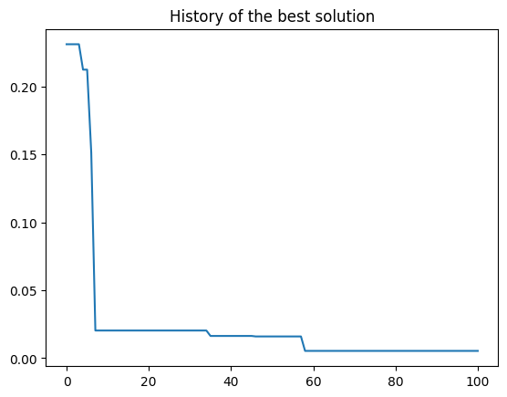
The minimum value is f(x) = 0.00538227051503521 at x = [1.06031746031746, 1.1284493284493284].
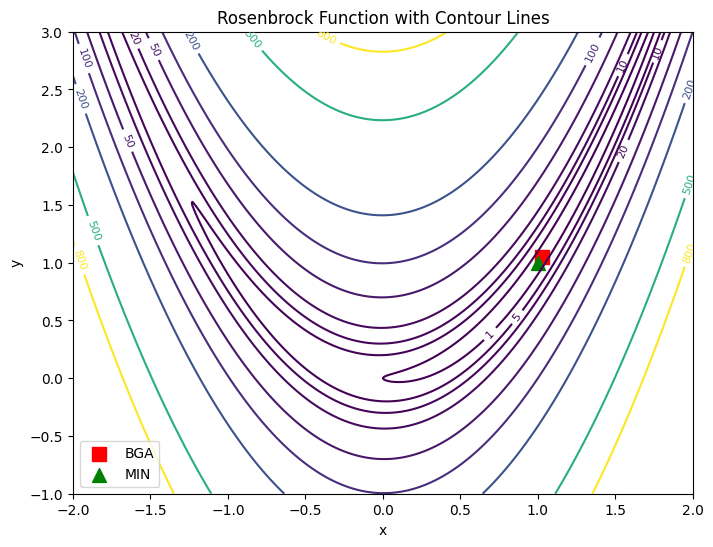
[18]:
import numpy as np
import matplotlib.pyplot as plt

# Generate grid data
x = np.linspace(-2, 2, 400)
y = np.linspace(-1, 3, 400)
X, Y = np.meshgrid(x, y)
Z = np.array([[Rosenbrock([xi, yi]) for xi, yi in zip(row_x, row_y)] for row_x, row_y in zip(X, Y)])

# Create the plot with contour lines
plt.figure(figsize=(8, 6))
levels = [0, 1, 5, 10, 20, 50, 100, 200, 500, 800]
contour = plt.contour(X, Y, Z, levels=levels, cmap='viridis')
plt.clabel(contour, inline=True, fontsize=8)
plt.title('Rosenbrock Function with Contour Lines')
plt.xlabel('x')
plt.ylabel('y')

x = result.phenotype
plt.scatter(x[0], x[1], color="red", s=100, marker='s', label="BGA")

plt.scatter(1, 1, color="green", s=100, marker='^', label="MIN")

plt.legend()
plt.show()
Just like for linear programming, you can use the Function class to pose problems using symbolic functions.
[19]:
variables = sy.symbols("x y")
obj = Function("(1-x)**2 + 100*(y-x**2)**2", variables=variables)
ranges = [[-2, 2], [-1, 3]]
bga = BGA(obj, ranges, length=12, nPop=100, minimize=True)
result = bga.solve()
result.phenotype, result.fitness
[19]:
([1.2224664224664226, 1.4986568986568987], 0.05128292180908297)